Product development
The concept of Data structures is most dreaded and avoided by programmers at the beginner level. In software engineering, Data structures provide solutions to a broad scope of problems. Making it essential to serve as a requirement for senior programming roles in most top technological companies.
What are Data Structures?
Data structures are specialised formats for storing, organising, managing, processing, and retrieving data for easy accessibility and modification. While there are different types of Data structures each one is universal across programming languages but with different syntax.
Why are Data Structures important?
A good understanding of data structures boosts a programmer’s ability to proffer detailed solutions to problems by sharing insights into individual usage of structures. The use of code and tools to develop digital products requires storing sets of information for proper referencing and modification, hence its importance in software engineering.
Common examples of features where Data structures are used include “Facebook friend lists”, “undo-redo feature of a text editor”, “Document-Object Model of a browser”, “text auto-complete feature”, among many other data features of a digital product.
Measuring The Efficiency of Data Structures
Determining the most suitable data structure to solve a problem requires measuring its speed and efficiency using the Big O Notation. The standard criteria for measuring data efficiency include a data’s ability to access, search, insert, and delete elements in the data structures.
The Big O Notation
To know the most suitable data structure to use, there is a need to measure the speed and efficiency of the data structure. The standard criteria considered in calculating this is the efficiency in accessing, searching, inserting, and deleting elements in the data structure. The Big O Notation is the conventional way to measure the efficiency of data structures.
Big O notations are recorded using Time Complexity Equations. Contrary to what the name suggests, the time complexity is not a measure of the actual time it takes the computer to carry out the function. It is actually a measure of the number of operations it takes to complete a function.
The time complexity equation of a function can be written as;
T(n) = O(x).
- Where T(n) is the time complexity.
- n is an integer representing the size or number of elements in the data structure.
- x is the number of operations required to completely execute the function on a data structure in respect to size n.
This equation is read as ‘a time complexity O of x’. Mostly, the number of elements in the data structure has a negative effect on the number of operations that need to be performed for the computer to carry out a function like searching through the data set. The worst-case scenarios are used when measuring the time complexity of a data structure, i.e., the highest possible number of n is considered. Confused? Check out the examples below.
Consider the types of time complexities below:
i. Constant Time Complexity
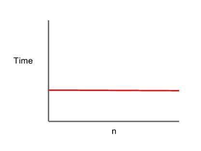
This means the number of operations carried out to execute the function is constant, irrespective of the size of the data structure. One element data set, and a quadrillion elements data set — the same number of operations. This is the best and most efficient Time Complexity Equation and is represented as T(n) = O(1).
ii. Logarithmic Time Complexity
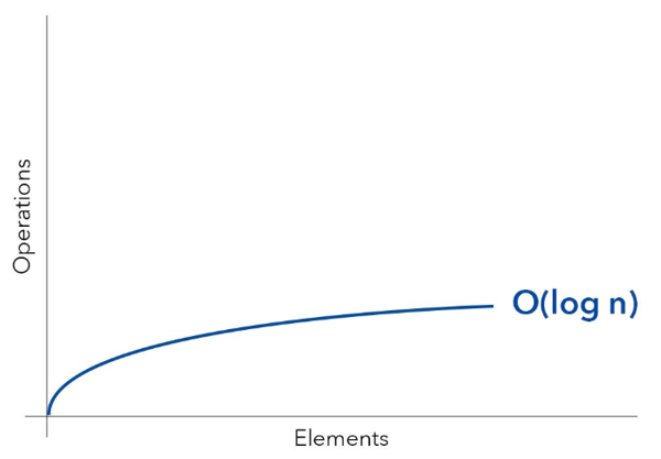
This means the number of operations carried out to execute the function increases logarithmically with the size of the data structure. It is slower than constant time complexity but still considered a fast time complexity. It is represented as T(n) = O(log n).
iii. Linear Time Complexity

This means as the size of the data structure increases, the number of operations carried out to execute the function increases at the same pace. This is considered a decent Time Complexity Equation and is represented as T(n) = O(n).
iv. Quadratic Time complexity
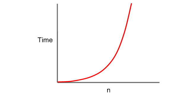
This means the number of operations carried out to execute the function is squared, with an increase in the size of the data structure. This is considered an inefficient Time Complexity Equation and is represented as T(n) = O(n²).
Some other time complexities include;
v. Log-Linear Time Complexity: T(n) = O(n log n).
vi. Exponential time: T(n) = O(cn), where c is some constant.
vii. Factorial time: T(n) =O(n!).
…
The above detailed types of time complexities directly work with each type of data structures. In this second part of this article, the basic types of data structures and individual time complexities are discussed. To find out more about data structures, click here.